13 - Parallel Query Execution

Background

Previous discussions of query executions assumed that the queries executed with a single worker (i.e thread). However, in practice, queries are often executed in parallel with multiple workers.

Parallel execution provides a number of key benefits for DBMSs: • Increased performance in throughput (more queries per second) and latency (less time per query). • Increased responsiveness and availability from the perspective of external clients of the DBMS. • Potentially lower total cost of ownership (TCO). This cost includes both the hardware procurement and software license, as well as the labor overhead of deploying the DBMS and the energy needed to run the machines. There are two types of parallelism that DBMSs support: inter-query parallelism and intra-query parallelism.

Parallel vs Distributed Databases

In both parallel and distributed systems, the database is spread out across multiple “resources” to improve parallelism. These resources may be computational (e.g., CPU cores, CPU sockets, GPUs, additional machines) or storage (e.g., disks, memory). It is important to distinguish between parallel and distributed systems. • Parallel DBMS In a parallel DBMS, resources, or nodes, are physically close to each other. These nodes communicate with high-speed interconnect. It is assumed that communication between resources is not only fast, but also cheap and reliable. • Distributed DBMS In a distributed DBMS, resources may be far away from each other; this might mean the database spans racks or data centers in different parts of the world. As a result, resources communicate using a slower interconnect over a public network. Communication costs between nodes are higher and failures cannot be ignored.

Even though a database may be physically divided over multiple resources, it still appears as a single logical database instance to the application. Thus, a SQL query executed against a single-node DBMS should generate the same result on a parallel or distributed DBMS.

Process Models

A DBMS process model defines how the system supports concurrent requests from a multi-user application/environment. The DBMS is comprised of more or more workers that are responsible for executing tasks on behalf of the client and returning the results. An application may send a large request or multiple requests at the same time that must be divided across different workers. There are two major process models that a DBMS may adopt: process per worker and thread per worker. A third common database usage pattern takes an embedded approach.

Process per Worker

The most basic approach is process per worker. Here, each worker is a separate OS process, and thus relies on OS scheduler. An application sends a request and opens a connection to the databases system. Some dispatcher receives the request selects one of its worker processes to manage the connection. The application now communicates directly with the worker who is responsible for executing the request that the query wants. This sequence of events is shown in Figure 1. Relying on the operating system for scheduling effectively reduces the DBMS’s control over execution. Further, this model depends on shared memory to maintain global data structures or relies on message passing, which has higher overhead. An advantage of the process per worker approach is that a process crash doesn’t disrupt the whole system because each worker runs in the context of its own OS process. This process model raises the issue of multiple workers on separate processes making numerous copies of the same page. A solution to maximize memory usage is to use shared-memory for global data structures so that they can be shared by workers running in different processes. Examples of systems that utilize the process-per-worker process model include IBM DB2, Postgres, and Oracle. When these DBMSs were developed, pthreads had not yet become the standard threading model. The semantics of threading varied from OS to OS while fork() was better defined.

Thread per Worker

The most common model nowadays is thread per worker. Instead of having different processes doing different tasks, each database system has only one process with multiple worker threads. In this environment, the DBMS has full control over the tasks and threads, it can manage it own scheduling. The multi-threaded model may or may not use a dispatcher thread. A diagram of the thread per worker model is shown in Figure 2. Using multi-threaded architecture provides certain advantages. For one, there is less overhead per context switch. Additionally, a shared model does not have to be maintained. However, the thread per worker model does not necessarily imply that the DBMS supports intra-query parallelism. Almost every DBMS created in the last 20 years uses this approach, including Microsoft SQL Server and MySQL. IBM DB2 and Oracle have updated their models to provide support for this apporach, as well. Postgres and Postgres-dervied databases largely still use the process-based approach.

Scheduling

In conclusion, for each query plan, the DBMS has to decide where, when, and how to execute. Relevant questions include: • How many tasks should it use? • How many CPU cores should it use? • What CPU cores should the tasks execute on? • Where should a task store its output? When making decisions regarding query plans, the DBMS always knows more than the OS and should be prioritized as such.

Embedded DBMS

A very different usage pattern for databases invovles running the system in the same address space of the application, as opposed to a client-server model where the database stands independent of the application. In this scenario, the application will set up the threads and tasks to run on the database system. The application itself will largely be responsible for scheduling. A diagram of an embedded DBMS’s scheduling behaviors is shown in Figure 3. DuckDB, SQLite, and RocksDB are the most famous embedded DBMSs.

Inter-Query Parallelism

In inter-query parallelism, the DBMS executes different queries are concurrently. Because multiple workers are running requests simultaneously, overall performance is improved. This increases throughput and reduces latency. If the queries are read-only, then little coordination is required between queries. However, if multiple queries are updating the database concurrently, more complicated conflicts arise. These issues are discussed further in lecture 15.

Intra-Query parallelism

In intra-query parallelism, the DBMS executes the operations of a single query in parallel. This decreases latency for long-running queries. The organization of intra-query parallelism can be thought of in terms of a producer/consumer paradigm. Each operator is a producer of data as well as a consumer of data from some operator running below it.

Parallel algorithms exist for every relational operator. The DBMS can either have multiple threads access centralized data structures or use partitioning to divide work up.

Within intra-query parallelism, there are three types of parallelism: intra-operator, inter-operator, and bushy. These approaches are not mutually exclusive. It is the DBMS’ responsibility to combine these techniques in a way that optimizes performance on a given workload.

Intra-Operator Parallelism (Horizontal)

In intra-operator parallelism, the query plan’s operators are decomposed into independent fragments that perform the same function on different (disjoint) subsets of data. The DBMS inserts an exchange operator into the query plan to coalesce results from child operators. The exchange operator prevents the DBMS from executing operators above it in the plan until it receives all of the data from the children. An example of this is shown in Figure 4.

In general, there are three types of exchange operators: • Gather: Combine the results from multiple workers into a single output stream. This is the most common type used in parallel DBMSs. • **Distribute: **Split a single input stream into multiple output streams. • **Repartition: **Reorganize multiple input streams across multiple output streams. This allows the DBMS take inputs that are partitioned one way and then redistribute them in another way.

Inter-Operator Parallelism (Vertical)

In inter-operator parallelism, the DBMS overlaps operators in order to pipeline data from one stage to the next without materialization. This is sometimes called pipelined parallelism. See example in Figure 5. This approach is widely used in stream processing systems, which are systems that continually execute a query over a stream of input tuples.

Bushy Parallelism

Bushy parallelism is a hybrid of intra-operator and inter-operator parallelism where workers execute multiple operators from different segments of the query plan at the same time. The DBMS still uses exchange operators to combine intermediate results from these segments. An example is shown in Figure 6.

I/O Parallelism

Using additional processes/threads to execute queries in parallel will not improve performance if the disk is always the main bottleneck. Therefore, it is important to be able to split a database across multiple storage devices. To get around this, DBMSs use I/O parallelism to split installation across multiple devices. Two approaches to I/O parallelism are multi-disk parallelism and database partitioning.

Multi-Disk Parallelism

In multi-disk parallelism, the OS/hardware is configured to store the DBMS’s files across multiple storage devices. This can be done through storage appliances or RAID configuration. All of the storage setup is transparent to the DBMS so workers cannot operate on different devices because the DBMS is unaware of the underlying parallelism.

RAID 是什么？

RAID （ Redundant Array of Independent Disks ）即独立磁盘冗余阵列，简称为「磁盘阵列」，其实就是用多个独立的磁盘组成在一起形成一个大的磁盘系统，从而实现比单块磁盘更好的存储性能和更高的可靠性。

RAID0

RAID0 是一种非常简单的的方式，它将多块磁盘组合在一起形成一个大容量的存储。当我们要写数据的时候，会将数据分为\(N\)份，以独立的方式实现\(N\)块磁盘的读写，那么这N份数据会同时并发的写到磁盘中，因此执行性能非常的高。 RAID0 的读写性能理论上是单块磁盘的\(N\)倍（仅限理论，因为实际中磁盘的寻址时间也是性能占用的大头） 但RAID0的问题是，它并不提供数据校验或冗余备份，因此一旦某块磁盘损坏了，数据就直接丢失，无法恢复了。因此RAID0就不可能用于高要求的业务中，但可以用在对可靠性要求不高，对读写性能要求高的场景中。

RAID1

RAID1 是磁盘阵列中单位成本最高的一种方式。因为它的原理是在往磁盘写数据的时候，将同一份数据无差别的写两份到磁盘，分别写到工作磁盘和镜像磁盘，那么它的实际空间使用率只有50%了，两块磁盘当做一块用，这是一种比较昂贵的方案。

RAID1其实与RAID0效果刚好相反。RAID1 这种写双份的做法，就给数据做了一个冗余备份。这样的话，任何一块磁盘损坏了，都可以再基于另外一块磁盘去恢复数据，数据的可靠性非常强，但性能就没那么好了。

RAID5

因为 RAID5 是一种将 存储性能、数据安全、存储成本 兼顾的一种方案。 在了解RAID5之前，我们可以先简单看一下RAID3，虽然RAID3用的很少，但弄清楚了RAID3就很容易明白RAID5的思路。 RAID3的方式是：将数据按照RAID0的形式，分成多份同时写入多块磁盘，但是还会另外再留出一块磁盘用于写「奇偶校验码」。例如总共有\(N\)块磁盘，那么就会让其中额度\(N-1\)块用来并发的写数据，第\(N\)块磁盘用记录校验码数据。一旦某一块磁盘坏掉了，就可以利用其它的\(N-1\)块磁盘去恢复数据。 但是由于第\(N\)块磁盘是校验码磁盘，因此有任何数据的写入都会要去更新这块磁盘，导致这块磁盘的读写是最频繁的，也就非常的容易损坏。 RAID5的方式可以说是对RAID3进行了改进。 RAID5模式中，不再需要用单独的磁盘写校验码了。它把校验码信息分布到各个磁盘上。例如，总共有\(N\)块磁盘，那么会将要写入的数据分成\(N\)份，并发的写入到\(N\)块磁盘中，同时还将数据的校验码信息也写入到这\(N\)块磁盘中（数据与对应的校验码信息必须得分开存储在不同的磁盘上）。一旦某一块磁盘损坏了，就可以用剩下的数据和对应的奇偶校验码信息去恢复损坏的数据。 RAID5校验位算法原理：\(P = D1 \oplus D2 \oplus D3 … \oplus Dn\) （D1,D2,D3 … Dn为数据块，P为校验，xor为异或运算） RAID5的方式，最少需要三块磁盘来组建磁盘阵列，允许最多同时坏一块磁盘。如果有两块磁盘同时损坏了，那数据就无法恢复了。

RAID6

为了进一步提高存储的高可用，聪明的人们又提出了RAID6方案，可以在有两块磁盘同时损坏的情况下，也能保障数据可恢复。 为什么RAID6这么牛呢，因为RAID6在RAID5的基础上再次改进，引入了双重校验的概念。 RAID6除了每块磁盘上都有同级数据\(XOR\)校验区以外，还有针对每个数据块的\(XOR\)校验区，这样的话，相当于每个数据块有两个校验保护措施，因此数据的冗余性更高了。 但是RAID6的这种设计也带来了很高的复杂度，虽然数据冗余性好，读取的效率也比较高，但是写数据的性能就很差。因此RAID6在实际环境中应用的比较少。

RAID10

RAID10其实就是RAID1与RAID0的一个合体。我们看图就明白了：

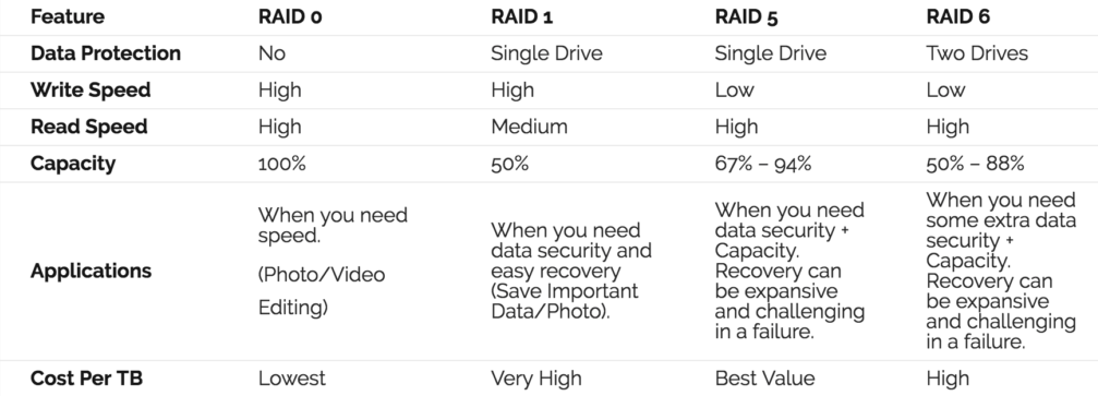
RAID10兼备了RAID1和RAID0的有优点。首先基于RAID1模式将磁盘分为2份，当要写入数据的时候，将所有的数据在两份磁盘上同时写入，相当于写了双份数据，起到了数据保障的作用。且在每一份磁盘上又会基于RAID0技术讲数据分为N份并发的读写，这样也保障了数据的效率。 但也可以看出RAID10模式是有一半的磁盘空间用于存储冗余数据的，浪费的很严重，因此用的也不是很多。 整体对比一下 RAID0、RAID1、RAID5、RAID6、RAID10 的几个特征：

Database Partitioning

In database partitioning, the database is split up into disjoint subsets that can be assigned to discrete disks. Some DBMSs allow for specification of the disk location of each individual database. This is easy to do at the file-system level if the DBMS stores each database in a separate directory. The log file of changes made is usually shared.

The idea of _logical partitioning _is to split single logical table into disjoint physical segments that are stored/managed separately. Such partitioning is ideally transparent to the application. That is, the application should be able to access logical tables without caring how things are stored. The two approaches to partitioning are vertical and horizontal partitioning. In vertical partitioning, a table’s attributes are stored in a separate location (like a column store). The tuple information must be stored in order to reconstruct the original record. In horizontal partitioning, the tuples of a table are divided into disjoint segments based on some partitioning keys. There are different ways to decide how to partition (e.g., hash, range, or predicate partitioning). The efficacy of each approach depends on the queries. We will cover these approaches later in the semester when discussing distributed databases.